This article shows how to make a graph showing a Linux machine’s swap memory. This plugin gathers physical swap memory utilization – cached, free, and used. In general, this module collects simple data for the swap memory like the Linux command free. The purpose of this article is to make a graph showing swap memory usage and consumption.
The Linux machine is using collectd to gather the swap memory statistics and send them to the time series back-end – InfluxDB. Grafana is used to visualize the data stored in the time series back-end InfluxDB and organize the graphs in panels and dashboards. Check out the previous articles on the subject to install and configure such software to collect, store and visualize data – Monitor and analyze with Grafana, influxdb 1.8 and collectd under CentOS Stream 9, Monitor and analyze with Grafana, influxdb 1.8 and collectd under Ubuntu 22.04 LTS and Create graph for Linux CPU usage using Grafana, InfluxDB and collectd
The collectd daemon is used to gather data on the Linux system and to send it to the back-end InfluxDB.
Key knowledge for the Swap collectd plugin
- The collectd plugin Swap official page – https://collectd.org/wiki/index.php/Plugin:Swap
- The Swap plugin options – https://collectd.org/documentation/manpages/collectd.conf.5.shtml#plugin_swap This article relies on the default plugin’s options
<Plugin swap>
#       ReportByDevice false
#       ReportBytes true
#       ValuesAbsolute true
#       ValuesPercentage false
#       ReportIO true
</Plugin>
All the devices are reported as a single device not per device and bytes and absolute values are used not percentages.
- to enable the Swap plugin, load the plugin with the load directive in /etc/collectd.conf
LoadPlugin swap
- The Swap plugin collects data every 10 seconds.
- swap_value – includes a single Gauge value under swap type – a metric, which value that can go up and down. It is used to count the swap occupancy for the different categories (the category is saved in a tag value of one record, and the categories are free, used and etc.). So there are multiple gauge values with different tags for the different swap categories at a given time. And a second counter under swap_io type
tag key tag value description host server hostname The name of the source this measurement was recorded. type swap | swap_io swap is the type, which will group the swap usage categories (cached, free, used). The swap_io groups the swap IO usage – how many IO operations are executed (in, out). type_instance swap categories The categories are cached, free, used. - A Gauge value – a metric, which value that can go up and down. More on the topic – Data sources.
A GAUGE value is simply stored as-is. This is the right choice for values which may increase as well as decrease, such as temperatures or the amount of memory used.
- A DERIVE value – a metric, in which the change of the value is interesting. For example, it can go up indefinitely and it is important how fast it goes up, there are functions and queries, which will give the user the derivative value.
These data sources assume that the change of the value is interesting, i.e. the derivative. Such data sources are very common with events that can be counted, for example, the number of emails that have been received per second by an MTA since it was started. The total number of emails is not interesting.
- To cross-check the value, the user can use the /proc/swap, /proc/meminfo and /proc/vmstat
[root@srv ~]# cat /proc/swaps
Filename                                Type            Size    Used    Priority
/dev/zram0                              partition       16777212        2533856 -1
[root@srv ~]# cat /proc/meminfo |egrep -e "^(SwapTotal:|SwapFree:|SwapCached:)"
SwapCached:       175416 kB
SwapTotal:      16777212 kB
SwapFree:       14202396 kB
[root@srv ~]# cat /proc/vmstat |egrep -e "^(pswpout|pswpin)"
pswpin 877611681
pswpout 376878365
The swap_io values are multiplied by the page size of the current system. For Linux, it is 4K. Note, by default, the ReportBytes collectd option is not enabled, so the swap_io measurement is in pages since the last reboot. The swap_io counter is read from the pswpout and pswpin (i.e. they also represent the pages since the last reboot). In fact, these two values are really important to track down because they tell how much the system touches swap device(s) and it could point out a problem with the physical memory shortages.
The InfluxQL queries for the Linux Swap plugin are grouped by where the swap is used (cached, free, used).
The queries are Grafana generated.
SELECT mean("value") FROM "swap_value" WHERE ("host" = 'srv2' AND "type" = 'swap') AND $timeFilter GROUP BY time($__interval), "type_instance" fill(null)
The mean function will compute the mean if there is more than one value in the database for every 10 seconds (this is the “group by” logic here). Probably the most accurate query might be to use the last() function instead of mean() and to group by time(10s) (or the time interval, of which the data is written in the database). As mentioned above, the collectd interval is 10 seconds. The function non_negative_derivative is needed to compute the difference between the values.
The query for the derived counter is a little bit complex.
SELECT non_negative_derivative(mean("value"), 1s) *4 FROM "swap_value" WHERE ("host" = 'srv2' AND "type" = 'swap_io') AND $timeFilter GROUP BY time($__interval), "type_instance" fill(null)
This query computes the difference every second because the swap_io counter stores the number of pages since the last reboot. And this number only increases, but the much more meaningful is to know how much data flows per second!
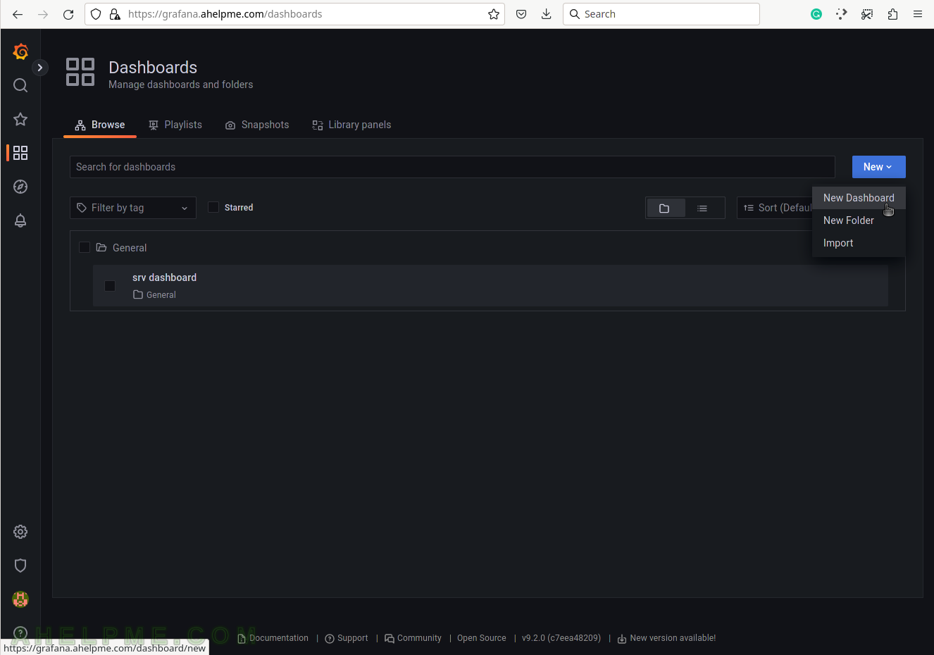
SCREENSHOT 1) Create a new dashboard, which will contain the Swap usage graph.
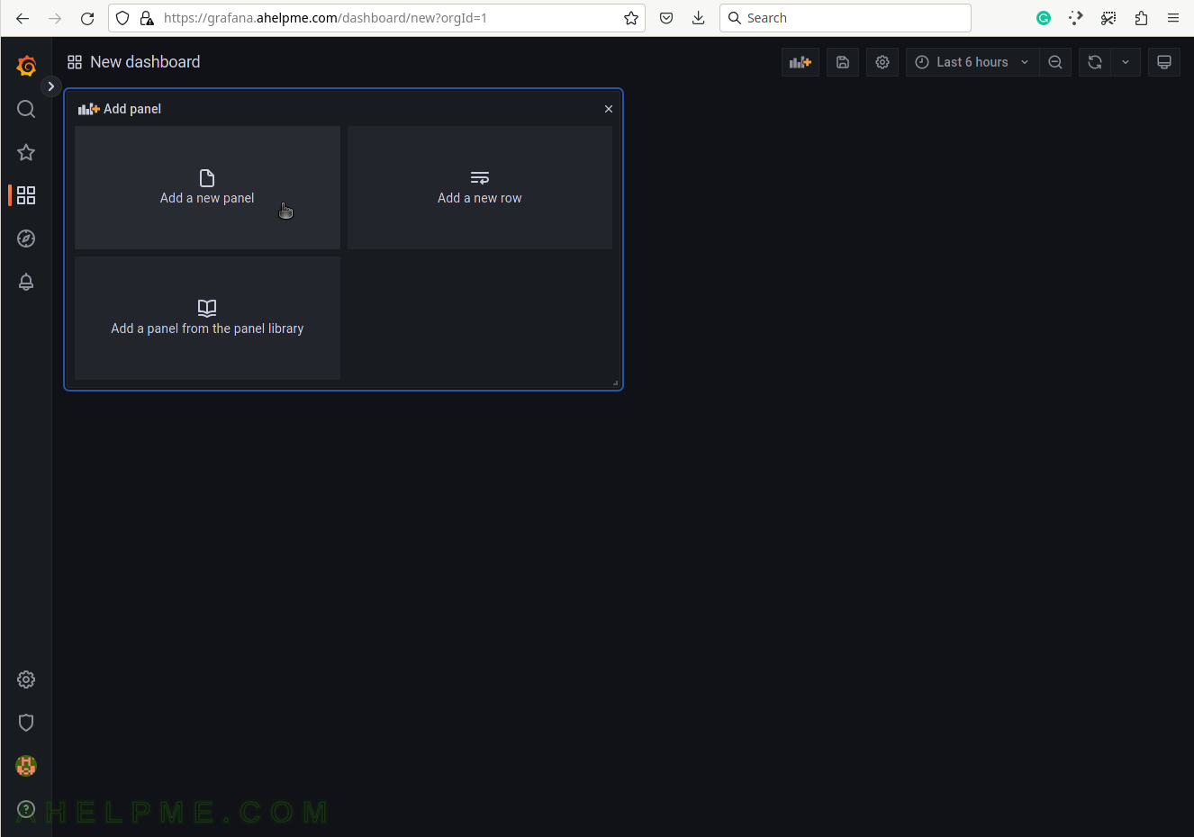
SCREENSHOT 2) Add a new panel in the new dashboard, which will contain the Swap usage graph.
SCREENSHOT 3) Change the “Data Source” to the collectd (InfluxDB) database and ensure on the right top the graph type is “Time series”.
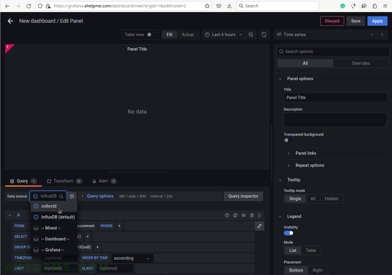
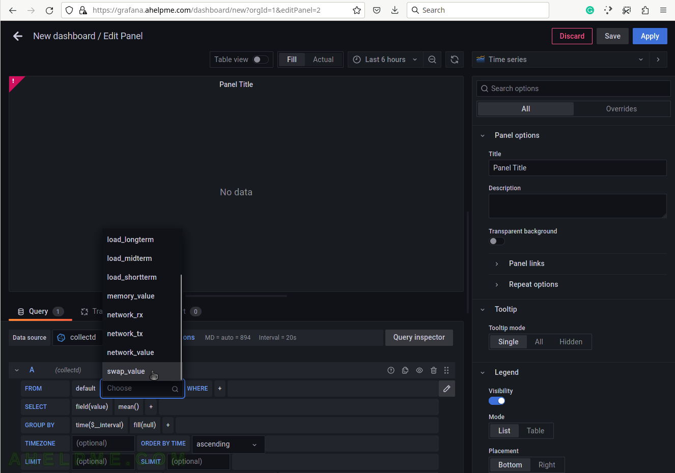
SCREENSHOT 4) Choose the swap_value from the measurement drop-down list.
There are all measurements in the drop-down list in the database collectd.
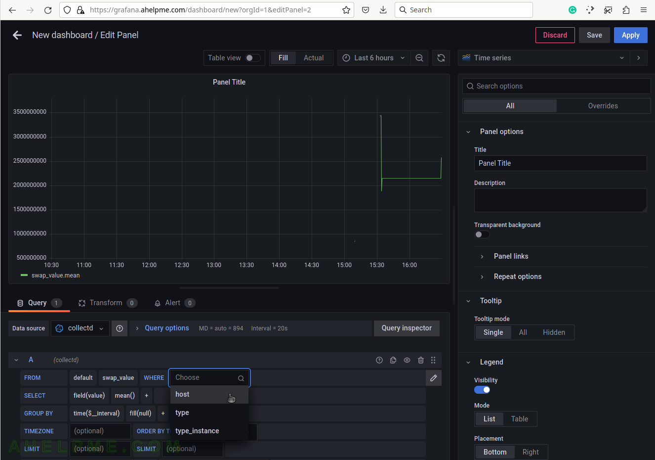
SCREENSHOT 5) Select the tag name “host” to limit the query for a selected hostname.
A tag is a key-value pair, which represents the metadata of a measurement record. For example, a measurement record consists of the actual measurement value and metadata for it such as which did the measurement and where. The server hostname “srv2” is the tag value and the tag key is the “host” name of the tag.
SCREENSHOT 6) Select the tag value “srv2”.
This setup has only one server, so no other servers’ hostnames are shown.

SCREENSHOT 7) Select the type of measurement.
Yet another measurement metadata. The type of measurement is swap, i.e. swap usage. There is an additional swap_io, which will be used for a graph later in this article. swap_io is used for a graph about the input and output IO, which the swap Linux kernel is doing.
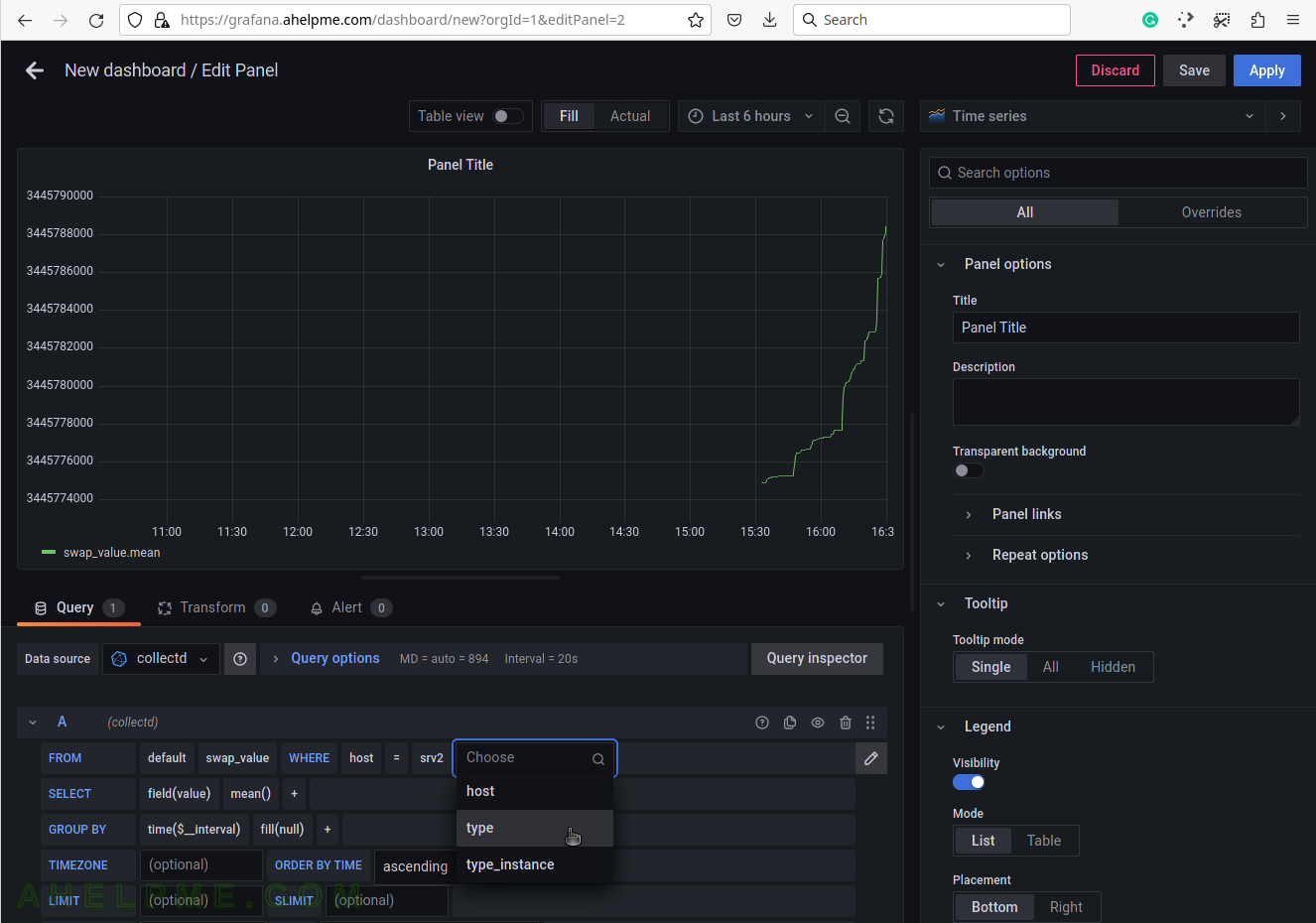
SCREENSHOT 8) Select swap for the tag value to draw swap usage in the graph.
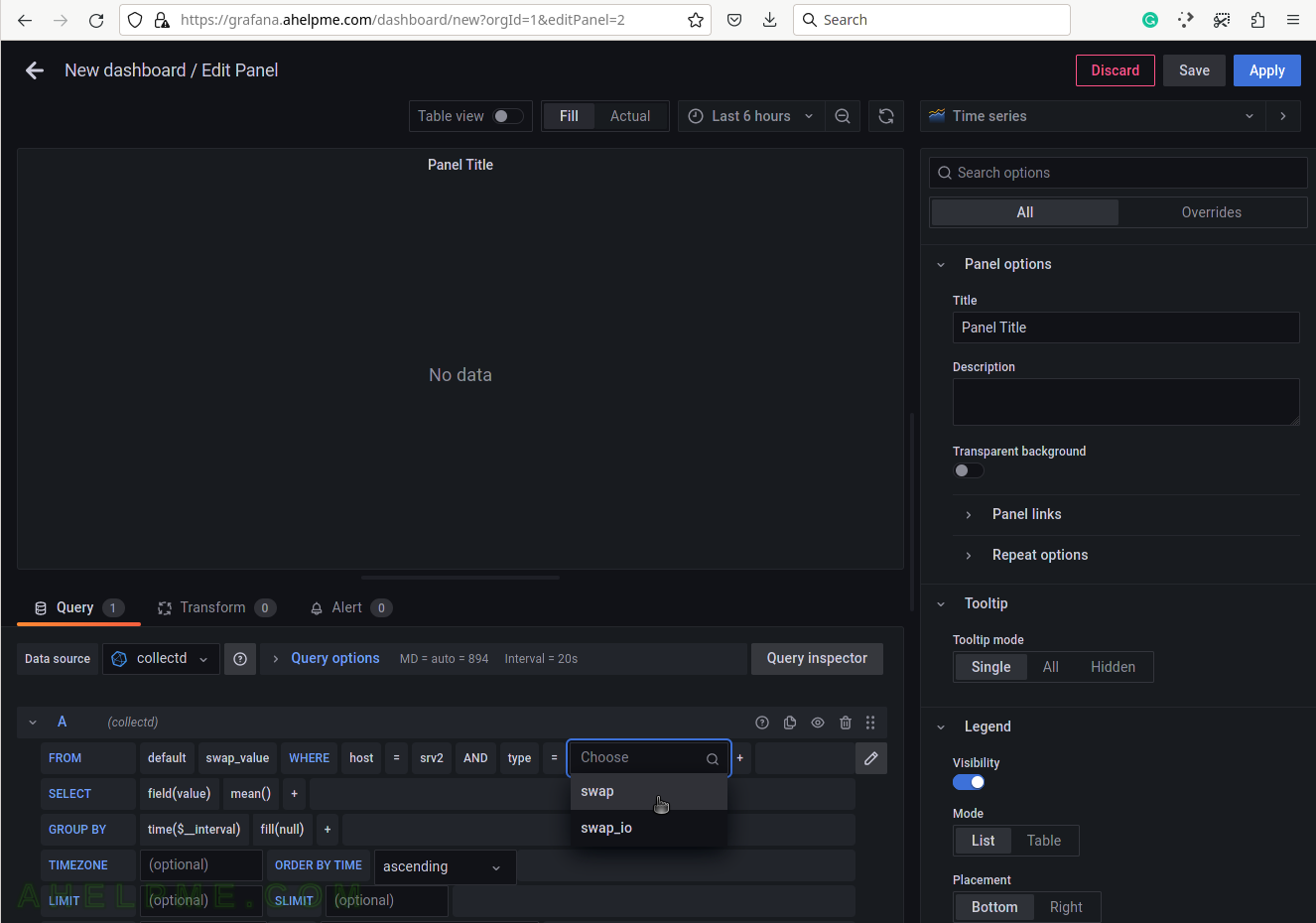
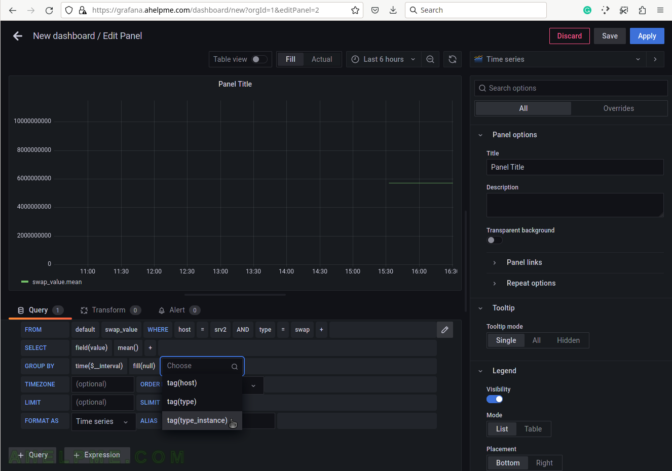
SCREENSHOT 9) Add a group by tag_instance to split the different tags in the graph.
The tag_instance shows the swap usage, which could be: cached, free, and used.
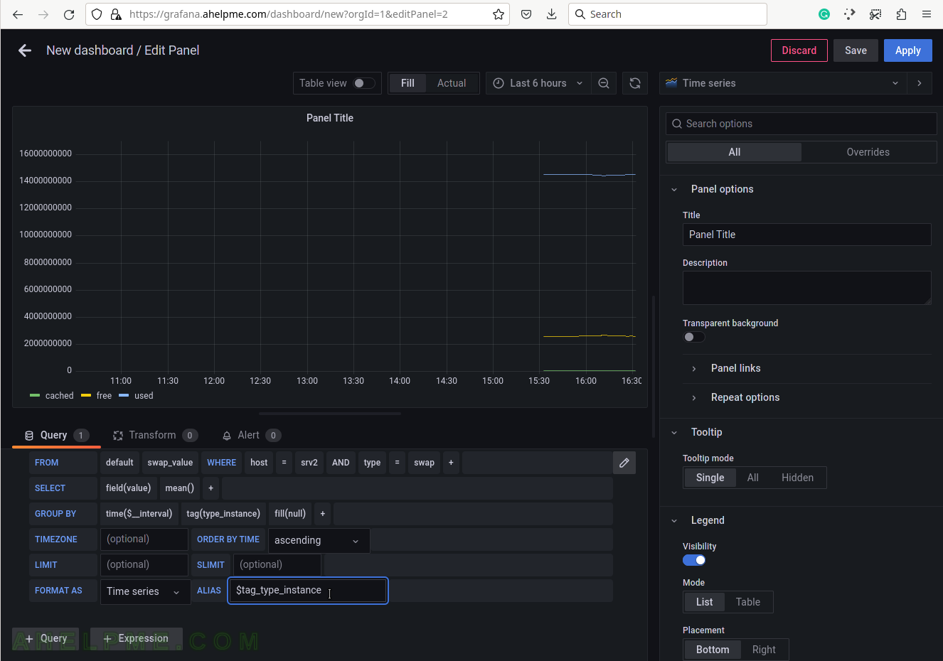
SCREENSHOT 10) To give pretty names to the tags in the graph’s legend add to the ALIAS a variable $tag_[tag_key] and in this case, the tag key is type_instance so that the variable will be $tag_type_instance.
There is an important variable “$__interval“, which may be edited and set to the rate of the original data (if applicable, not really for the swap usage) or left as is to be computed each time based on the selected time frame of the graph (6 hours for this example).