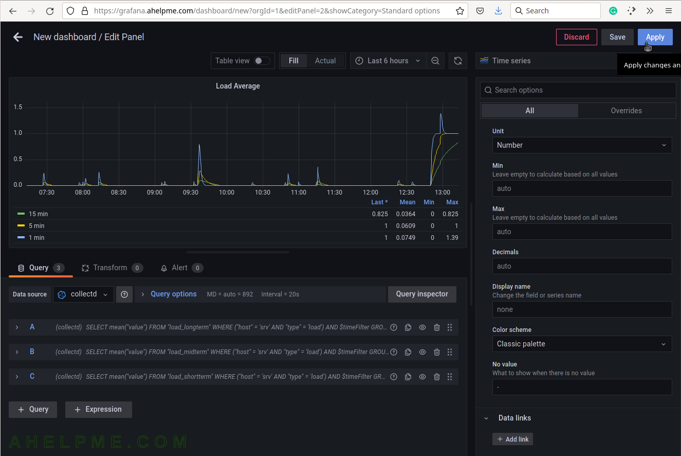
SCREENSHOT 21) Apply the changes in Edit panel.
Click on the top right corner button “Apply”.
SCREENSHOT 22) The Load average graph is ready.
Click on sub-menu “View” to expland it.
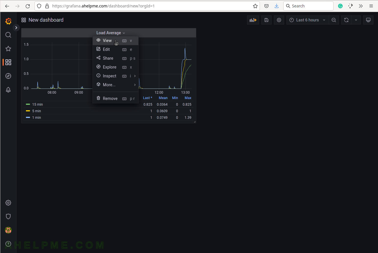
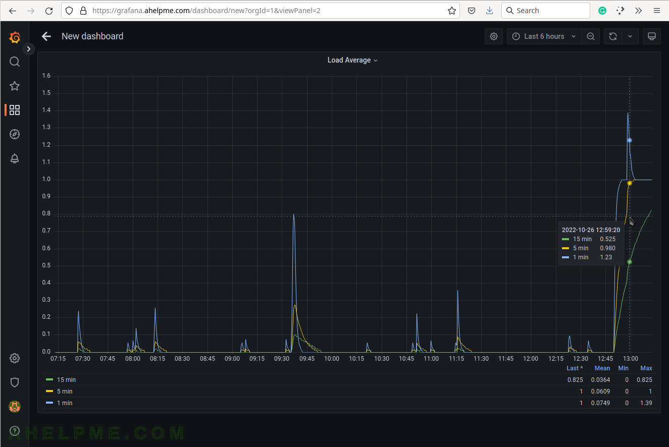
SCREENSHOT 23) There is a View menu, which will bring the graph as full page graph.
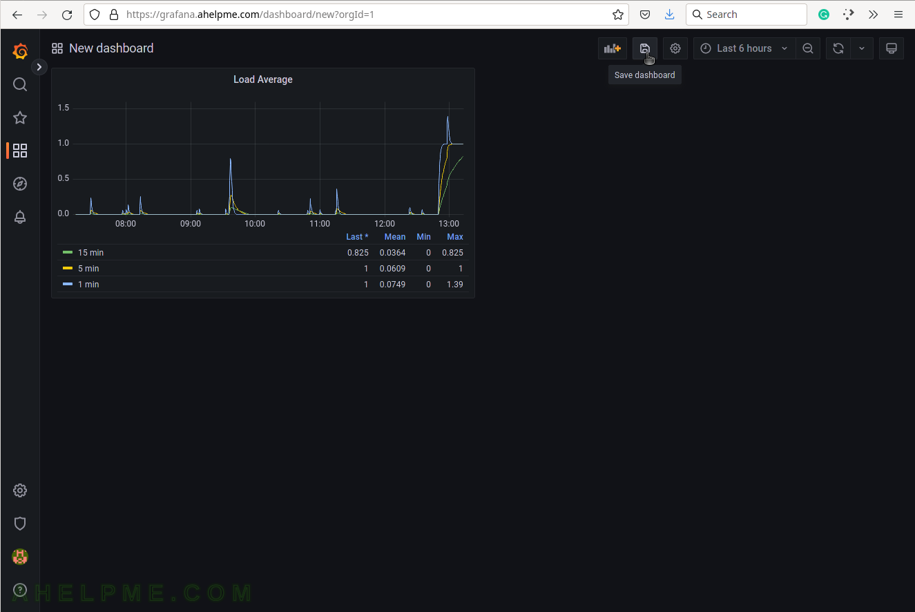
SCREENSHOT 24) Save the dashboard after exiting the View graph mode.
The save button is upper right.
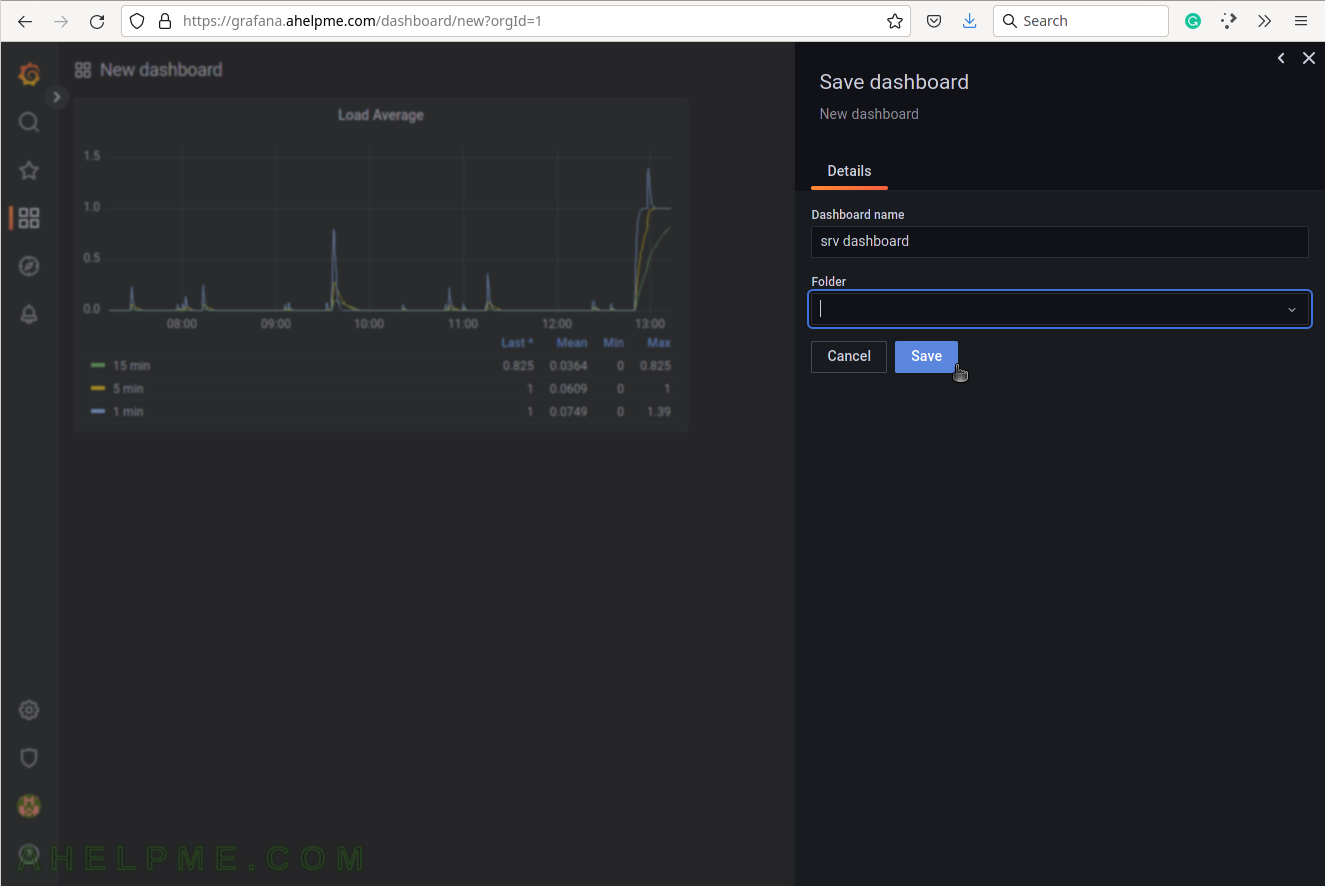
SCREENSHOT 25) Set the dashboard’s name and folder.
Click on “Save” to save all the graphs and the panel data of the newly created dashboard.
SCREENSHOT 26) Change the size of the panel if needed by hovering and clicking on the panel’s right bottom.
Move the mouse and the panel and the graph will expand.
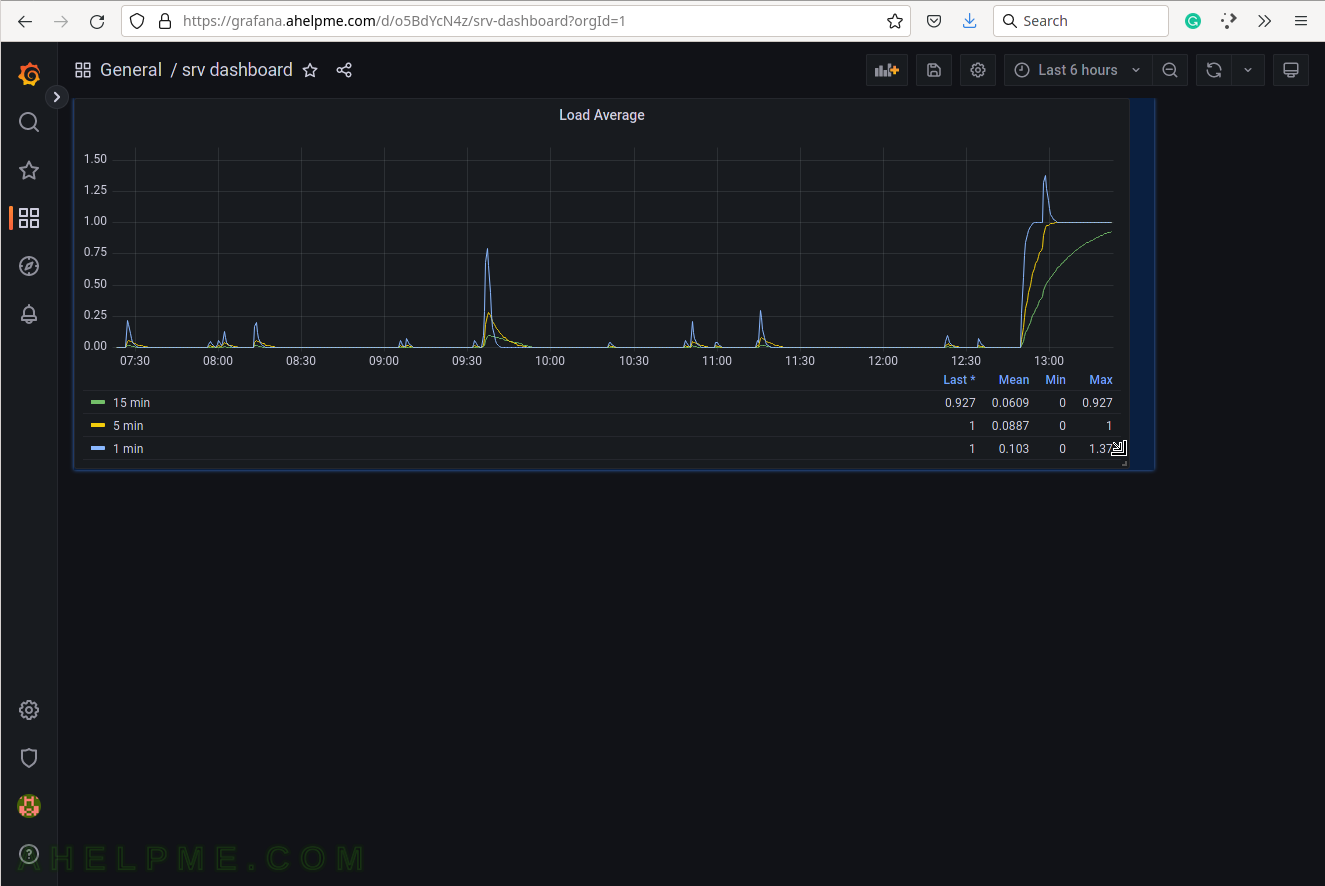
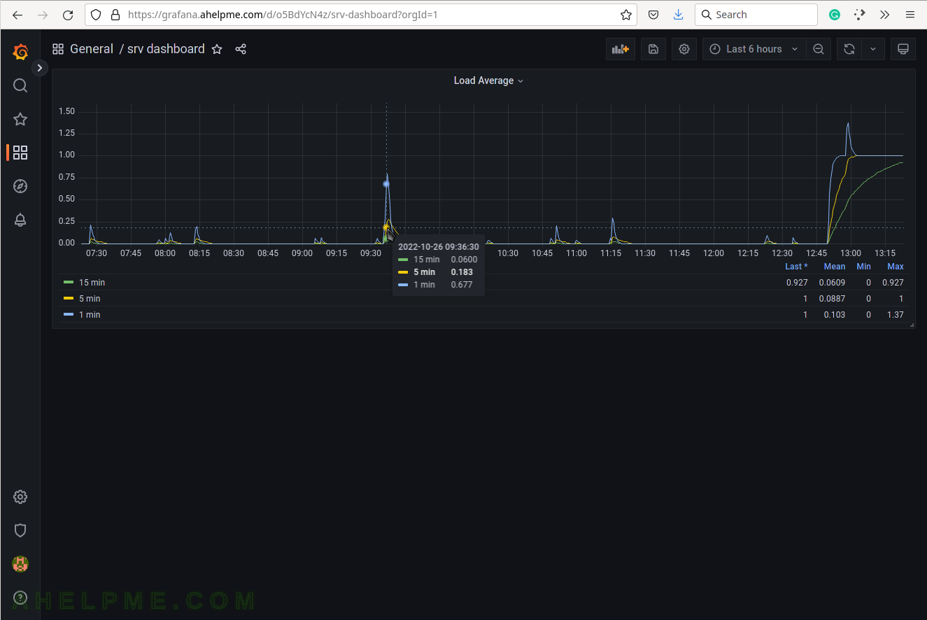
SCREENSHOT 27) The final look of the Load average graph.
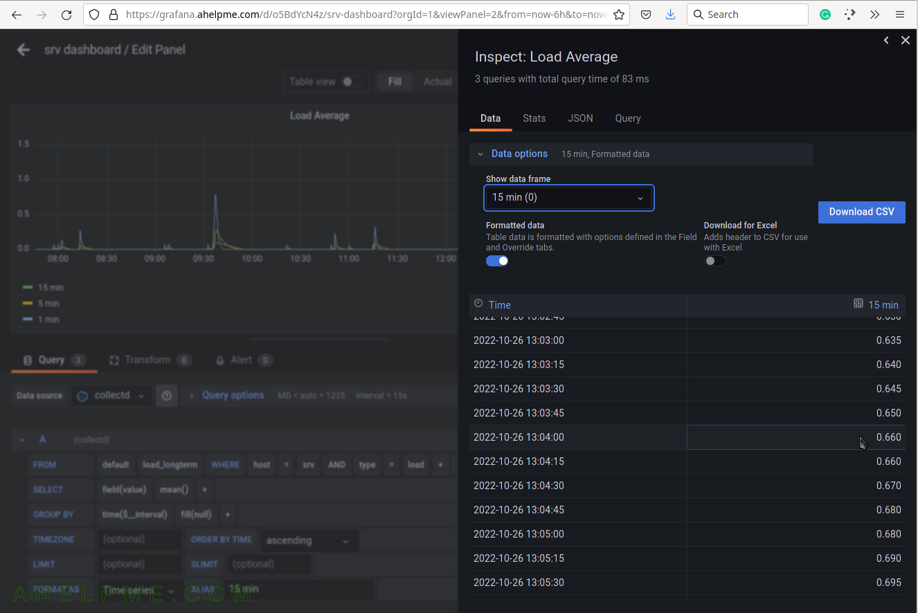
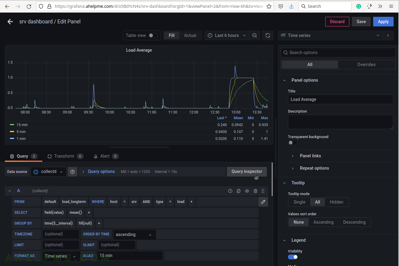
SCREENSHOT 28) Click on “Query Inspector” to see the values behind the graph and the query results or the real query sent to InfluxDB.
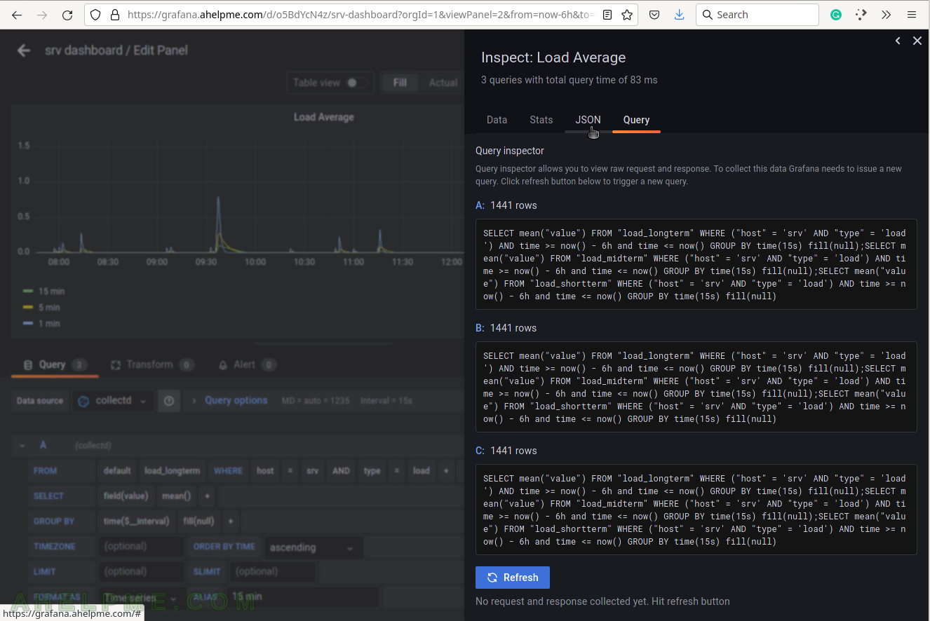
SCREENSHOT 29) The three queries in InfluxQL language, which are sent to the InfluxDB.
Some of the values are replaced with their real values such as “$__interval“, which is based on what time frame is selected – “Last 6 hours”.
SCREENSHOT 30) The Data tab in Query Inspector shows real values from the queries in a table form.